LAI Lab

When we look at engagement data, we usually ask a simple question:

Are students engaged or not?
Are they paying attention or distracted?

In reality, engagement is richer and more complex than a single score. A student can look attentive in class but feel emotionally disconnected. Another can feel very invested but struggle to organise their work. If we treat all of them as “high” or “low” engagement, we lose essential nuance.

In this article, I share a method to uncover those hidden patterns, using a technique called latent profile analysis.

Instead of asking “How engaged is the class?” it asks a different question:

“What kinds of engagement patterns exist in this class, and how many groups of students show those patterns?”

This article is the first part of a two-part series. In Part 1, I focus on the ideas. In Part 2, I walk through a simple tutorial in Python using real data. The goal of this first part is to build intuition and vocabulary so that the code in Part 2 feels less mysterious 🙂

This series is inspired by a tutorial chapter on latent profile analysis from the book Learning Analytics Methods and Tutorials, specifically Chapter 9, “An Introduction and R Tutorial to Model-based Clustering in Education via Latent Profile Analysis” (Scrucca et al., 2024). In that chapter, the authors work in R; here, I recreate the same workflow in Python, adapting it to my own approach.

Let us start with the data!

The data for this project comes from a study of primary school students in northern Spain, using a dataset described in López-Pernas et al. (2024). Researchers asked hundreds of students to complete the School Engagement measure (Fredricks et al., 2005), which captures three dimensions of engagement using a questionnaire: behavioral, emotional, and cognitive. The items cover behaviours such as paying attention, completing work, trying hard, and following rules (behavioral); whether students like school (emotional); and whether they are thoughtful and reflective when working (cognitive). Each item is rated on a Likert scale from 1 (not at all true) to 5 (very true).

From these items, we can calculate three engagement scores for each student: behavioral, emotional, and cognitive. Once we have those scores, it is tempting to summarise everything with a few averages.

If we look only at averages, the class might look something like this: behavioral engagement is fairly high on average, emotional engagement is moderate, and cognitive engagement is a bit lower. That summary is useful, but it raises a deeper question:

“Are there certain combinations that appear again and again in different students?”

For example, are there students who behave very well but do not feel emotionally connected? Are there students who feel good and are active, but do not invest much cognitively? Are there small groups who struggle on all three dimensions?

Latent variable models are designed exactly for this kind of question.

What are latent variable models?

Sometimes the things we want to study cannot be measured directly. You cannot put “motivation” or “anxiety” on a scale, but you can ask people questions and measure their answers. Latent variable models are a family of statistical models built for this situation. They assume that there are one or more hidden factors that we cannot observe directly, and that these factors influence the variables we can observe, such as test scores, survey answers, or behaviour logs.

These models have been in use for a long time across various fields.

In psychology, factor analysis has long been used to model general intelligence as a latent factor underlying many different test scores.

In the social sciences, structural equation models connect latent concepts such as attitudes or satisfaction to each other and to the survey items that measure them.

In natural language processing, topic models such as latent Dirichlet allocation treat topics as latent variables that generate the words we see, which helps uncover hidden themes in text.

In time series analysis, hidden Markov models describe unobserved states that evolve over time and generate the observed data.

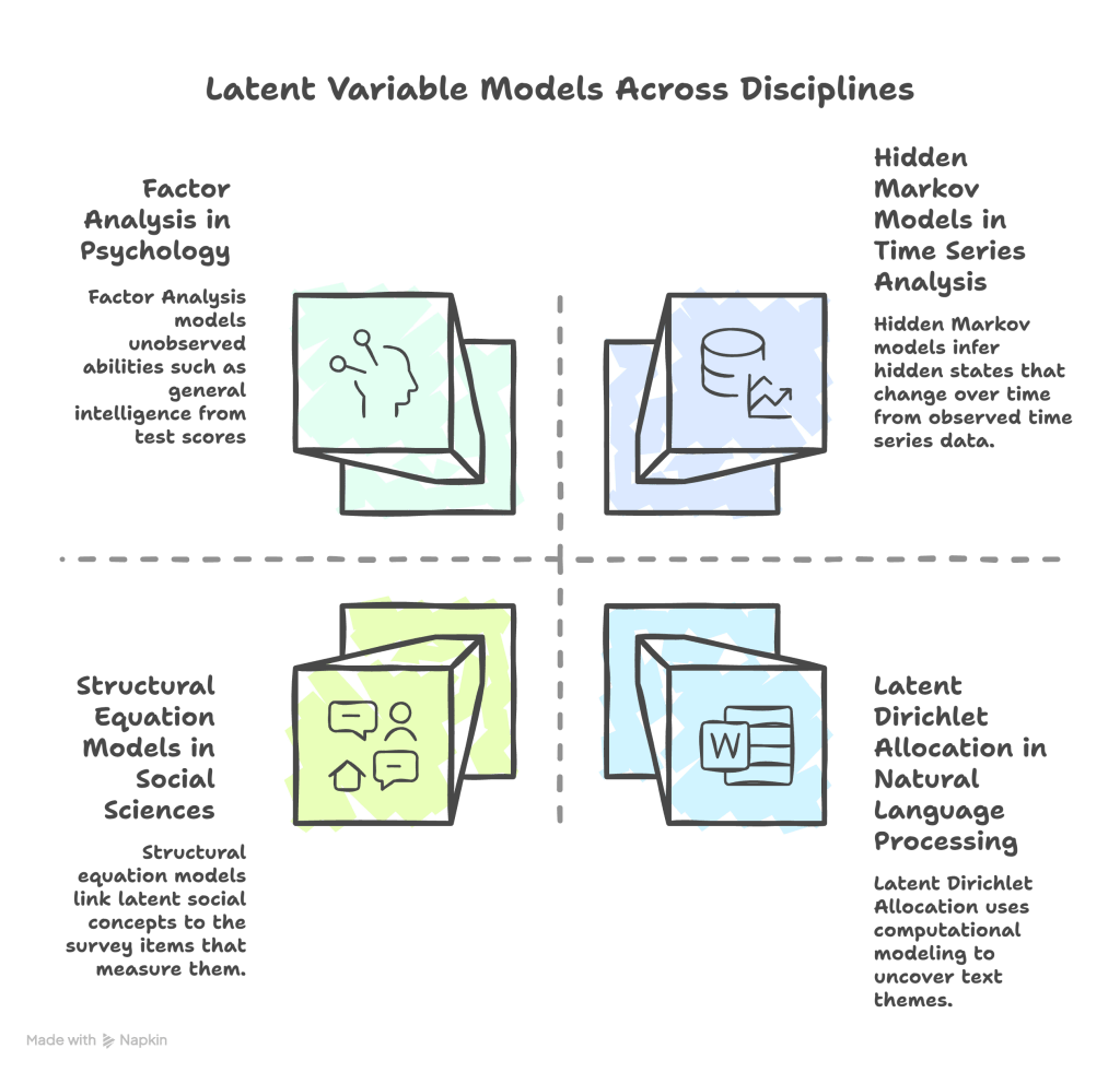
Across psychology, sociology, economics, biology, and many other fields, latent variable models help researchers make sense of complex phenomena that cannot be observed directly. Learning analytics is slowly joining that family, because many concepts that matter for learning, such as engagement or self-regulation, are also latent.

To understand where latent profile analysis fits, it is helpful to step back and look at the broader family of latent variable models. A simple way is to classify them by two questions:

What kind of variables we observe, and what kind of latent variables we assume.

Once we do that, latent profile analysis falls quite naturally into one specific box.

There is a simple way to organise this. First, ask whether the observed variables are continuous numbers or categories. Second, determine whether the latent variables are continuous numbers or categorical variables. Most common models fall into one of four combinations.

• If both the observed and latent variables are continuous, we get factor analysis.
• If the observed variables are categorical, for example, correct or incorrect answers, and the latent variable is continuous, for example, ability, we get a latent trait model, often called an item response theory model.
• If the observed variables are continuous and the latent variables are categorical, such as cluster membership, we obtain a latent profile model.
• If both the observed and latent variables are categorical, we get a latent class model.

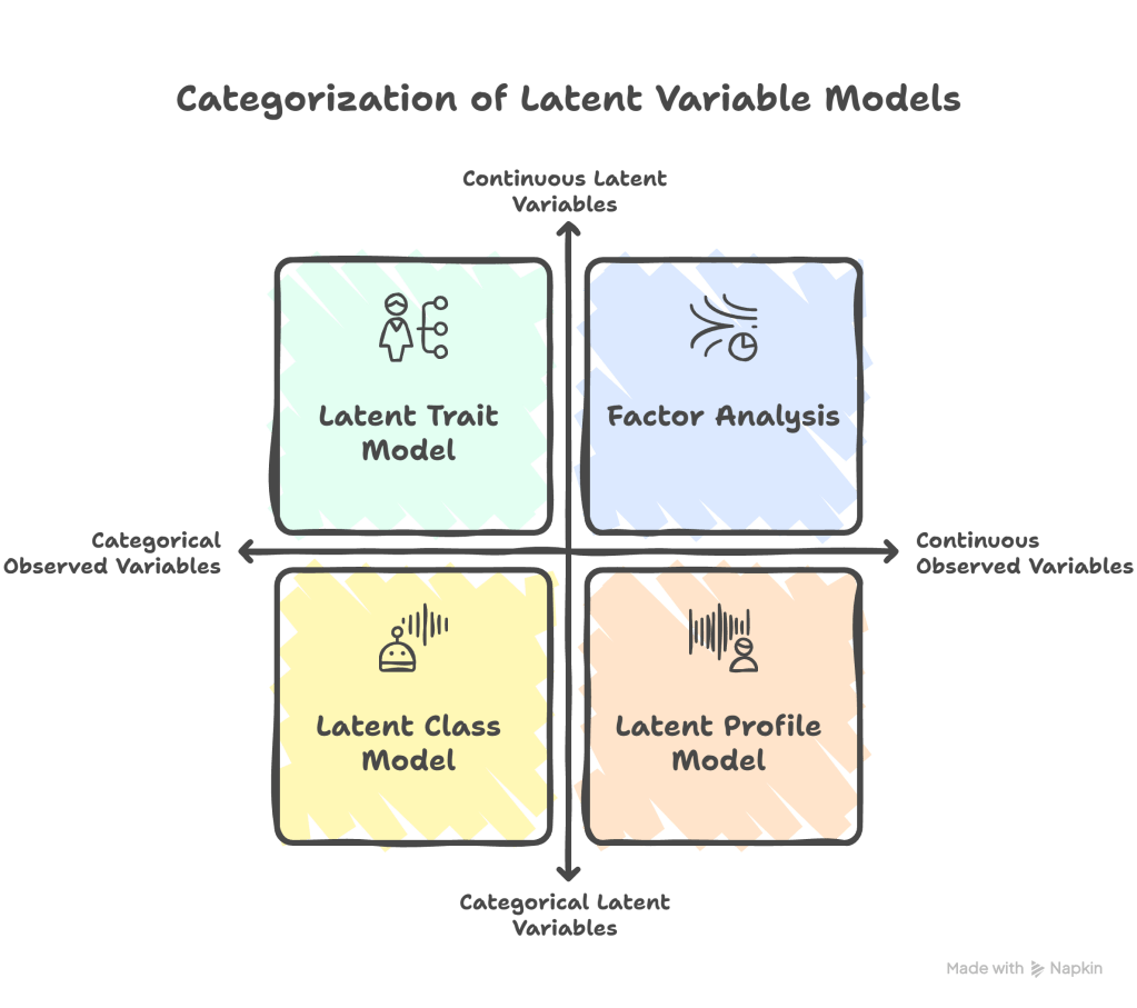
The latent profile model is the focus of this series (represented by the orange box in the bottom right). We treat the engagement scores (observed variables) as continuous numbers, and we assume that there are a few hidden categories of students (latent variables), which we call profiles. Each profile represents a type of student with a characteristic pattern across the three engagement dimensions.

Once we define latent profile analysis as “continuous observed variables + categorical latent profiles,” the next question is how to actually fit such a model in practice. In many applications, including this one, that work is done by Gaussian mixture models. They may look like standard clustering tools at first glance. Still, under the hood, they are doing exactly what a latent profile model needs: treating each profile as a probability distribution over the engagement scores.

How Gaussian mixture models connect to Latent Profile Analysis

In this framework, Gaussian mixture models are a special case of latent profile analysis. They make two main assumptions.

First, the observed variables are continuous and are roughly normally distributed within each profile. In our example, this means that the three engagement dimensions are treated as continuous scores that follow a normal distribution within each profile.

Second, the latent variable is a categorical label that tells us which cluster or profile each student belongs to.

Put together, this means that each student is assumed to come from one of a few normal distributions in the space of engagement scores. Each distribution represents a profile with its own typical pattern of emotional, cognitive, and behavioral engagement. This is why Gaussian mixture models can be viewed as part of the latent profile analysis family.

In practice, this connection shows up in software. In R, the mclust package fits Gaussian mixture models with different covariance structures. Packages such as tidyLPA build on top of that and present the results using the language of profiles and latent classes, which is more familiar to researchers in education and psychology. Under the hood, the mathematics is the same, but the interface is tuned to how people think about learners.

In Part 2 of this series, we will explore how the same idea is implemented in two tools. The original R tutorial uses mclust. A Python version uses GaussianMixture from scikit learn. Both are fitting Gaussian mixtures. Both can be interpreted as latent profile analysis. The fun part is seeing how close their results are and what to do when they are not exactly the same.

References

Fredricks, J. A., Blumenfeld, P., Friedel, J., & Paris, A. (2005). School engagement. In K. A. Moore & L. H. Lippman (Eds.), What do children need to flourish? Conceptualizing and measuring indicators of positive development (pp. 305–321). Springer.

Scrucca, L., Saqr, M., López-Pernas, S., & Murphy, K. (2024). An introduction and R tutorial to model based clustering in education via latent profile analysis. In M. Saqr & S. López-Pernas (Eds.), Learning analytics methods and tutorials: A practical guide using R (pp. 285–317). Springer. https://doi.org/10.1007/978-3-031-54464-4_9

López-Pernas, S., Saqr, M., Conde, J., & Del-Río-Carazo, L. (2024). A broad collection of datasets for educational research, training, and application. In M. Saqr & S. López-Pernas (Eds.), Learning analytics methods and tutorials: A practical guide using R (pp. 17–66). Springer. https://doi.org/10.1007/978-3-031-54464-4_2

Figure 1: image generated by Google Gemini, December 1, 2025, in response to the prompt “create image that represent digital learning,” https://gemini.google.com.

Figure 2 and 3: both images are generated by Napkin.ai, December 8, 2025.